Dwell time analysis#
Dwell time extraction#
Dwell times can be extracted from the overall classification File.classification using the File.determine_dwells_from_classification method:.
[2]:
file.determine_dwells_from_classification(variable='FRET', selected=True, inactivate_start_and_end_states=True)
The method will create an additional .nc file named <filename>_dwells.nc.
The contents from this file can be obtained using:
[3]:
file.dwells
[3]:
<xarray.Dataset>
Dimensions:           (dwell: 43360)
Dimensions without coordinates: dwell
Data variables:
    molecule_in_file  (dwell) int32 0 0 0 0 0 0 0 ... 821 823 824 824 825 825
    file              (dwell) |S25 b'ssHJ1\\ssHJ1 TIRF 561 0001' ... b'ssHJ1\...
    molecule          (dwell) int64 0 0 0 0 0 0 0 ... 821 823 824 824 825 825
    state             (dwell) int8 -128 1 0 1 0 1 ... -128 -128 -128 -1 -128 -1
    frame_count       (dwell) int64 2 1 4 2 1 2 1 1 ... 4 2 8 400 354 46 167 233
    duration          (dwell) float64 0.245 0.1225 0.4899 ... 5.634 20.45 28.54
    mean_FRET         (dwell) float64 0.2086 0.3119 0.2062 ... 0.00134 0.03914
    number_of_states  (dwell) int32 2 2 2 2 2 2 2 2 2 2 ... 2 2 2 2 2 1 1 1 1 1
Attributes:
selected: TrueFor each dwell the following information is provided:
file: the file from which it originatesmolecule_in_file: the molecule index in the original filestate: the state of the dwellframe_count: the dwell duration in framesduration: the dwell duration in timemean_<variable_name>: the mean of the used variable
The dwells with positive states that are at the beginning or the end of a trace, or have a negative state neighbor, are inactivated (i.e. set to state -128) by default. This is done because the events are interrupted and the full dwell time cannot be observed. In case this is not desired, the inactivate_start_and_end_states argument can be set to False.
Dwell time analysis#
The dwell times can be analyzed from a file object using the File.analyze_dwells method. This produces a fit result in the form of an xarray Dataset, containing the fit values for each state, each fit and each component.
[4]:
_ = file.analyze_dwells(method='histogram_fit', number_of_exponentials=[1,2])
The dwell times are used to estimate the parameters of a single or multi-component exponential distribution
where \(\text{PDF}\) is the probability density function over time \(t\) and \(P_i\) is the fractional contribution and \(k\) the reaction rate of the \(i\)-th component out of a total of \(n\) components.
The number of components can be indicated through the number_of_exponentials argument.
There are three analysis methods available: - Maximum likelihood estimation - Histogram fit - Cumulative density function (CDF) fit
The analysis result is automatically saved in an <filename>_dwell_analysis.nc netcdf file and can be accessed through:
[5]:
file.dwell_analysis
[5]:
<xarray.Dataset>
Dimensions:               (state: 2, component: 2, fit: 2)
Coordinates:
  * state                 (state) int64 0 1
  * component             (component) int32 0 1
Dimensions without coordinates: fit
Data variables:
    P                     (state, fit, component) float64 1.0 nan ... 0.4664
    k                     (state, fit, component) float64 2.487 nan ... 5.969
    truncation_min        (state, fit) float64 0.05803 0.06927 0.06052 0.06052
    P_error               (state, fit, component) float64 nan nan ... nan
    k_error               (state, fit, component) float64 1.604 nan ... 7.33e+05
    truncation_min_error  (state, fit) float64 0.1791 0.2913 0.04902 0.05991
    BIC                   (state, fit) float64 9.48e+04 9.438e+04 ... 5.865e+04
    number_of_components  (state, fit) int32 1 2 1 2
Attributes:
    papylio_version:                 0.0.0
    fit_function:                    exponential
    P_bounds:                        [-1  1]
    k_bounds:                        [1.e-09    inf]
    fit_method:                      histogram_fit
    bins:                            auto_discrete
    remove_first_bins:               0
    scipy_curve_fit_absolute_sigma:  True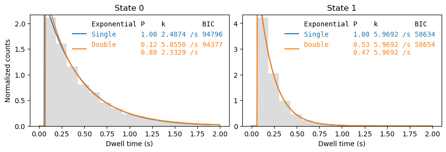
sampling_interval: 0.12248370927318296The fit result can be plotted using File.plot_dwell_analysis:
[6]:
fig, axes = plt.subplots(1,2, figsize=(9,3), layout='constrained')
_  = file.plot_dwell_analysis(plot_range=(0,2), axes=axes, log=False)
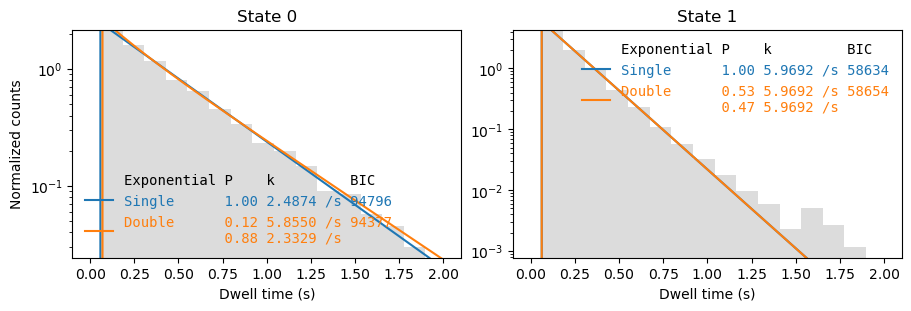
[7]:
fig, axes = plt.subplots(1,2, figsize=(9,3), layout='constrained')
_  = file.plot_dwell_analysis(plot_range=(0,2), axes=axes, log=True)
C:\Users\user\surfdrive\Promotie\Code\Python\papylio\papylio\analysis\dwell_time_analysis.py:840: UserWarning: Attempted to set non-positive bottom ylim on a log-scaled axis.
Invalid limit will be ignored.
  ax.set_ylim(0,counts.max()*1.03)
C:\Users\user\surfdrive\Promotie\Code\Python\papylio\papylio\analysis\dwell_time_analysis.py:840: UserWarning: Attempted to set non-positive bottom ylim on a log-scaled axis.
Invalid limit will be ignored.
  ax.set_ylim(0,counts.max()*1.03)
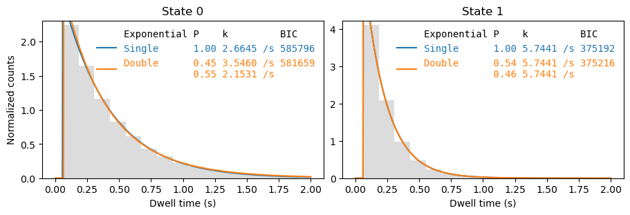
Combining data from multiple files#
[8]:
from papylio.analysis.dwell_time_analysis import analyze_dwells, plot_dwell_analysis

dwells = files.dwells
dwell_analysis = analyze_dwells(dwells, method='histogram_fit', number_of_exponentials=[1,2])

fig, axes = plt.subplots(1,2, figsize=(9,3), layout='constrained')
_ = plot_dwell_analysis(dwell_analysis, dwells, plot_type='pdf', plot_range=(0,2), axes=axes)